How we solved the Royal Game of Ur

We spent 7 years tinkering with AI for the Royal Game of Ur, and now we have strongly solved the Finkel, Blitz, and Masters rule sets! In the end, all it took was a couple pretty equations, which I will do my best to explain.

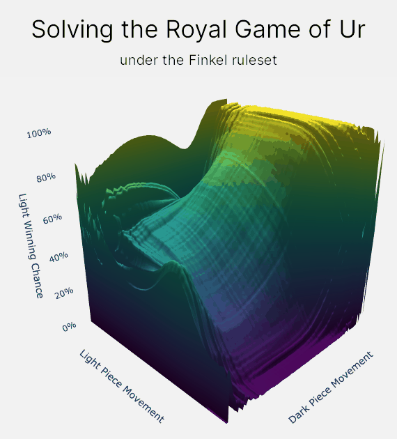
In fact, we have even gone beyond "just" strongly solving the game. Strongly solving the game requires us to find the best move from every position. We have done that, plus we have also calculated each player's precise chance of winning, under optimal play, from every position as well. All using our open-source library for the game, RoyalUr-Java.

Here's how it works! We have also written a technical report here.

Watch perfect play

Before we get into the details, here's a little live demo. Below, two bots engage in a flawless duel - perfect play! I find it mesmerising. How often do you get to watch something and know it is mathematically perfect?

⏷ Light's real-time chance of winning

Perfect play of the Royal Game of Ur between two bots. The dice are hidden to make the game quicker. You can play the perfect bot yourself here.

Perfection means maximising your chance of winning

In order to create a bot that plays perfectly, we need to create a bot that maximises its chance of winning.

Unlike in Chess or Go, when you play Ur you cannot plot a perfect victory in advance. The dice would never allow it! This makes solving the Royal Game of Ur fundamentally different to solving games without chance.

Instead of plotting out one single path to victory, we need to consider every possible future path, each enabled or disabled by the roll of the dice, and weigh them all in our choice of moves. This focus on weighing up future options makes solving the Royal Game of Ur more similar to solving Poker than to solving Chess.

We use value iteration to handle the chance

So, how do we possibly figure out what move maximises our chance of winning, especially when we might be 100s of moves from the end of the game? Our answer is to use value iteration.

Value iteration allows us take advantage of the Royal Game of Ur's relatively low number of states. For example, the Finkel rule set has only 276 million states. This is small enough that we can store the entire state graph for the Finkel rule set in memory. And then we can use value iteration to propagate your chance of winning or losing backwards through the entire game.

Above is a simplified example of how value iteration works to update a graph. Value flows from state to state, originally from the win or loss states, and then backwards towards the start of the game. In this example, the value that each state settles on is the chance of you ending up in the win state if you took a random walk from that point.

On larger graphs, like the graph for the Royal Game of Ur, I prefer to think of value iteration as a fluid simulation. "Winning chance" is the fluid, and it slowly flows backwards through the entirety of the Royal Game of Ur. And the especially neat thing is that the chances that value iteration settles on are your chance of winning!

An animation showing the process of calculating the light player's winning chance over a game of the Royal Game of Ur. — An animation showing the process of calculating the light player's winning chance from every position in the game.

How does value iteration actually work?

Here is the core idea of value iteration: we propagate wins and losses backwards.

Here is the intuition: If you know how good the next positions you might reach are, then you can calculate how good your current position is. And if you know how good that position is, you can calculate how good the positions before it are, and so on...

Using this method, we can work backwards through the entire game, updating the value of states based upon the states that come after them.

The backwards pass

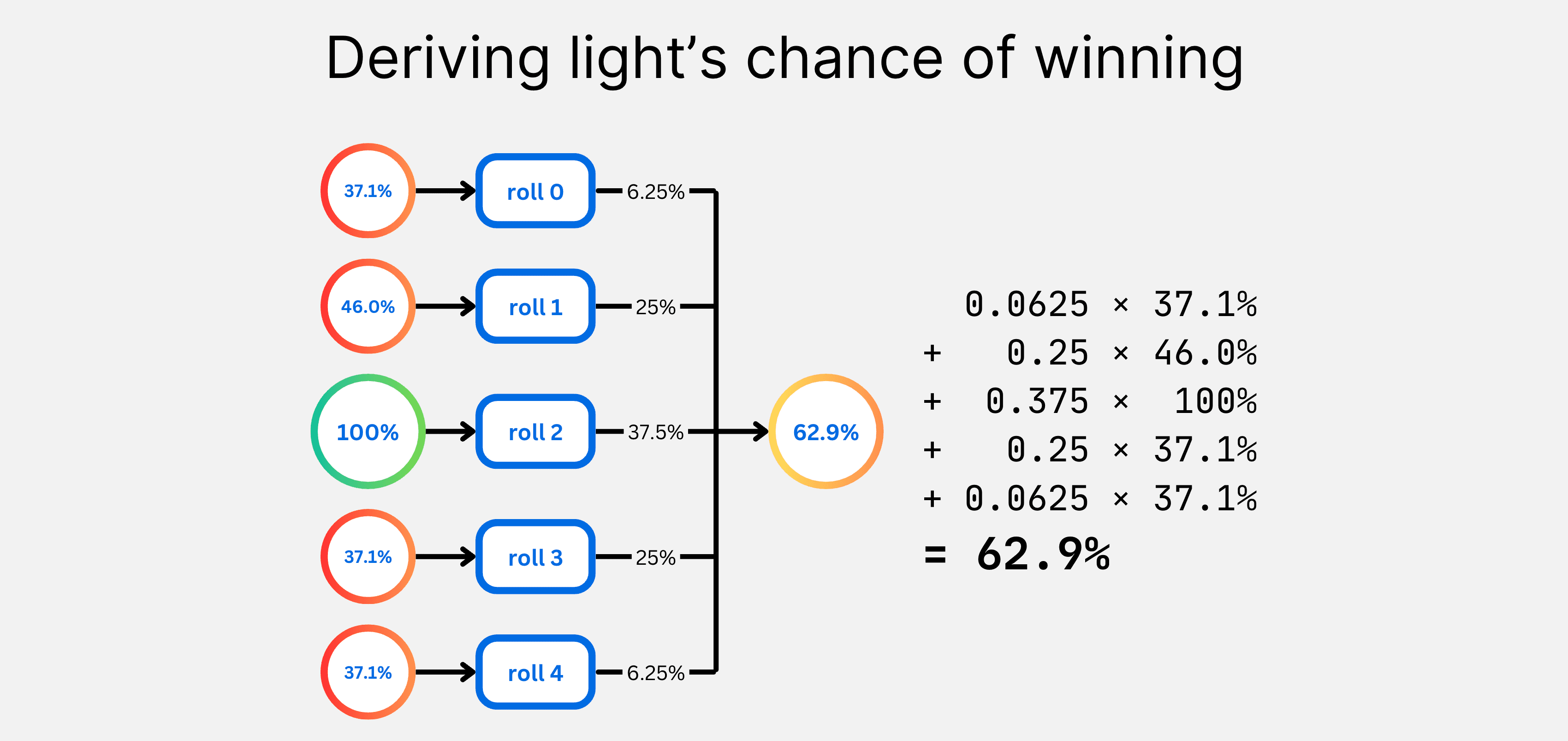
This "backwards pass" is implemented using a simple weighted average. Your chance of winning in one state is equal to the weighted average of your chance of winning in all the states you could reach after each roll of the dice (ignoring move selection for now).

V(\text{state}) = \sum_{\text{roll} \in \text{rolls}} \text{P(roll)} \cdot V(\text{state after roll \& best move})

This simple operation acts as the means by which wins and losses cascade through the state space of the Royal Game of Ur.

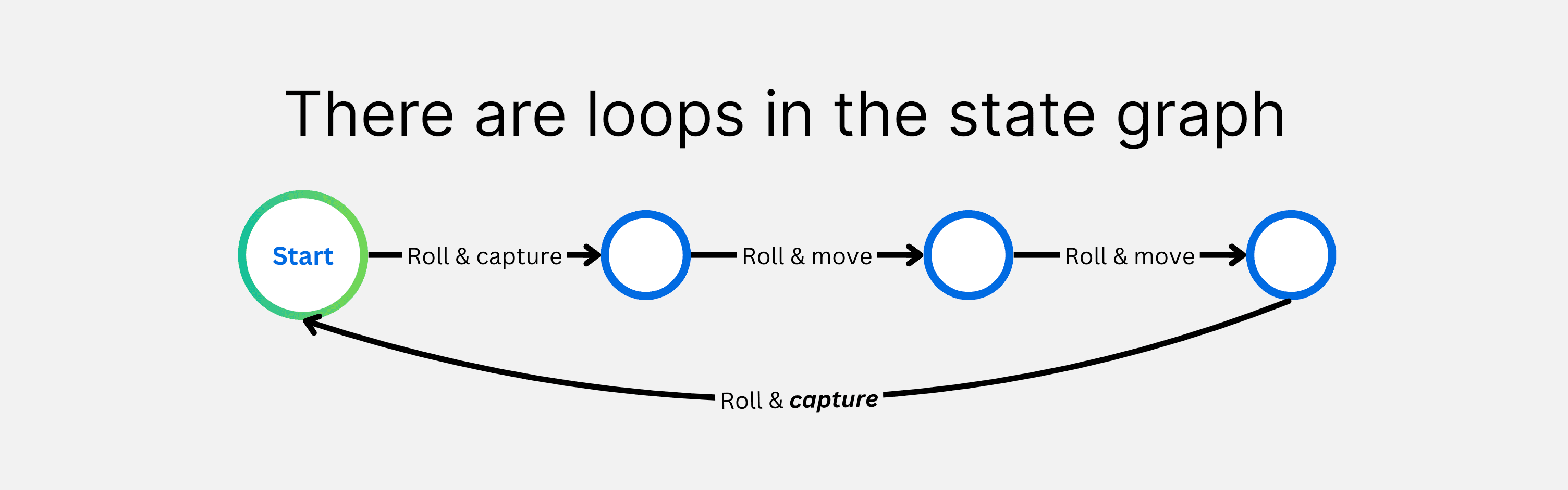
So is that all we need? Unfortunately, not quite. Loops in the state graph stop one backwards pass from being enough. There are pesky positions where it is possible to play a number of moves and get back to the same position as before we played them. The primary value of value iteration lies in solving these loops.

Deriving your chance of winning in one position based upon its neighbour positions that you would reach after each roll. — Deriving your chance of winning in one position based upon the neighbour positions you would reach after each roll of the dice.

We need to do lots of backwards passes

The iteration part of value iteration is how we deal with loops. Instead of doing one backwards pass, we will do many. On every backwards pass we do, our estimates for your chance of winning from each position will improve.

The reason loops cause a single backwards pass to be insufficient is because the win percentage of some states will be incorrect when you try to use them to calculate the winning chance of another state. Their value is incorrect because that state you just calculated can influence the states you used in the calculation (a circular dependency)!

A diagram showing how a capture of a piece can lead to a loop in the states that are visited in a game.

And it turns out, the equations we use here have been proven to converge over time. We know this because the equations we use to solve the Royal Game of Ur are formulations of the Bellman equations. And the Bellman equations have been mathematically proven to converge over time.

How do we consider what moves people make?

This is a crucial detail! And it links to a limitation of solving any game containing chance.

In any game containing chance, the best strategy to win depends heavily on what your opponent does. However, we cannot predict every individual player's quirks and tendencies. So instead, we assume that both players play optimally, making the best possible move at every turn.

By making the assumption that players play optimally, it means that we calculate a strategy where neither player can improve their chance of winning by changing their moves. This type of strategy is called a Nash Equilibrium. A strategy that is impossible to beat. But also a strategy that does not necessarily notice and exploit the weaknesses in your opponent's play. This is a tradeoff we make.

It turns out that a simple greedy approach is all you need to calculate optimal play. At each state, we assume that the player would make the move that leads to their highest chance of winning. Even though the win percentages you are using to make this decision might be incorrect at first, this is still good enough to let the win percentages converge over time.

Within our value iteration kernel, the selection of the optimal move for each player is represented by a maximum or minimum over the value of their possible moves.

V_{\text{light}}(\text{state}, \text{roll}) = \max_{\text{move} \in \text{moves}} \Bigl(V(\text{state after roll \& move})\Bigr)

V_{\text{dark}}(\text{state}, \text{roll}) = \min_{\text{move} \in \text{moves}} \Bigl(V(\text{state after roll \& move})\Bigr)

Final overview of value iteration

So, we have now seen how we might calculate the value of one state based upon other states. Let's bring this home with an explanation of how those pieces come together into a final set of equations, and how we actually apply them to create a solved game map.

The weighted average and move selection come together to form a simple kernel. This kernel combines the weighted average with our optimal move selection. We iteratively apply this kernel over all the states in the game, over and over again, until the win percentages converge. When applying this kernel, we use it to update values of $V(\text{state})$ in a map, using other values from the same map.

V(\text{state}) = \begin{cases} V_{\text{light}}(\text{state}), & \text{if the current player is light},\\ V_{\text{dark}}(\text{state}), & \text{if the current player is dark}. \end{cases}

V_{\text{light}}(\text{state}) = \sum_{\text{roll} \in \text{rolls}} \text{P(roll)} \cdot \max_{\text{move} \in \text{moves}} \Bigl(V(\text{state after roll \& move})\Bigr)

V_{\text{dark}}(\text{state}) = \sum_{\text{roll} \in \text{rolls}} \text{P(roll)} \cdot \min_{\text{move} \in \text{moves}} \Bigl(V(\text{state after roll \& move})\Bigr)

The map of states and values is our final output. The final map that is produced will contain our estimates for each player's chance of winning from every position. We can then use this map to make an agent play optimally, by making our agent pick the move that leads to a state with your highest chance of winning.

And that's it for value iteration! Value iteration has allowed us to solve the Royal Game of Ur down to an accuracy that is only limited by 64-bit floating point accuracy. For the Finkel rule set, that means calculating winning chances down to an accuracy around 3E-14%, or 0.00000000000003%. I find that to be super awesome :D

Now, let's make it fast! It's optimisation time.

The process that value iteration goes through to find the perfect solution to a game. — The process that value iteration goes through to find the perfect solution to the Royal Game of Ur.

Chop the game up for speed!

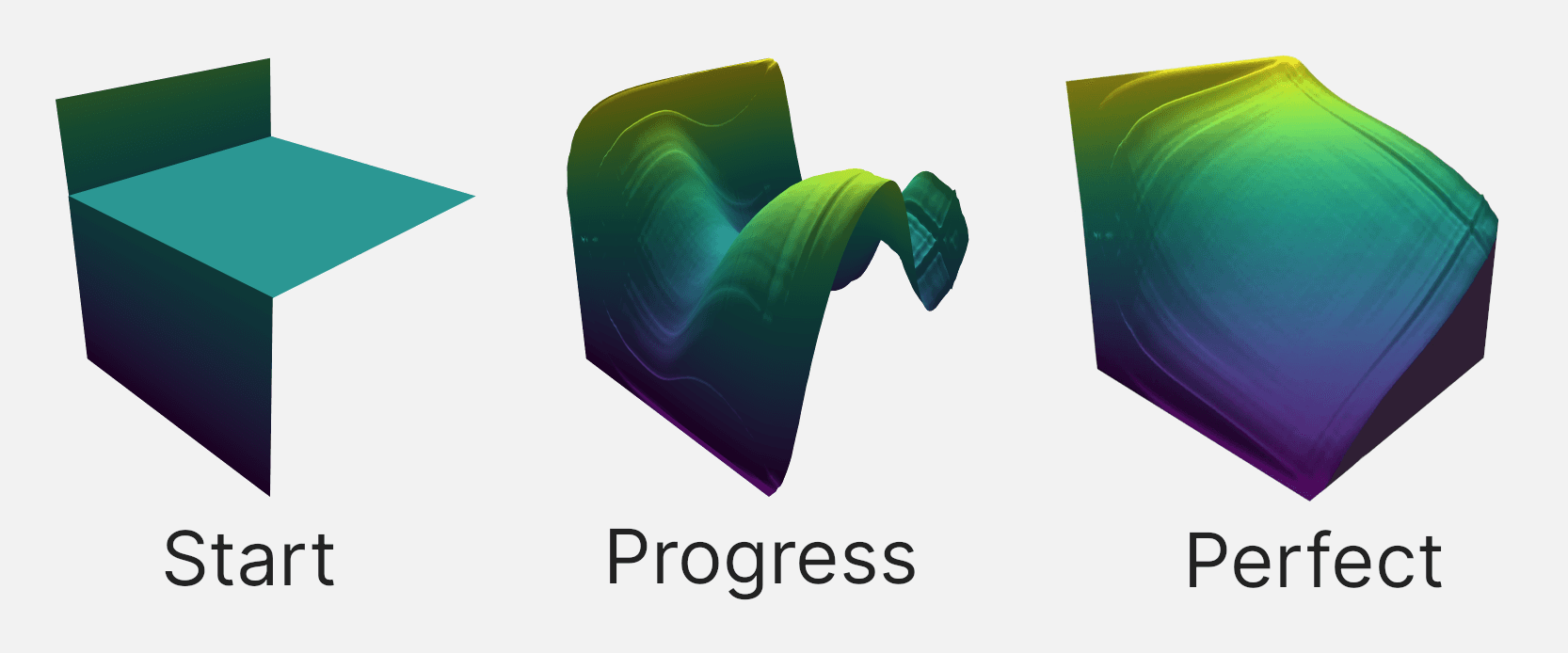
Performing value iteration on the entire game at once is expensive, and inefficient. During the thousand iterations it takes to train our models, there is really only a narrow boundary of states that are converging to their true value at a time. States closer to the winning states have already converged, and states further away don't have good enough information to converge yet.

We'd really love to only update the states that are close to converging in every iteration, to avoid wasting time updating everything else. Luckily, we have one delicious little trick that lets us do just that!

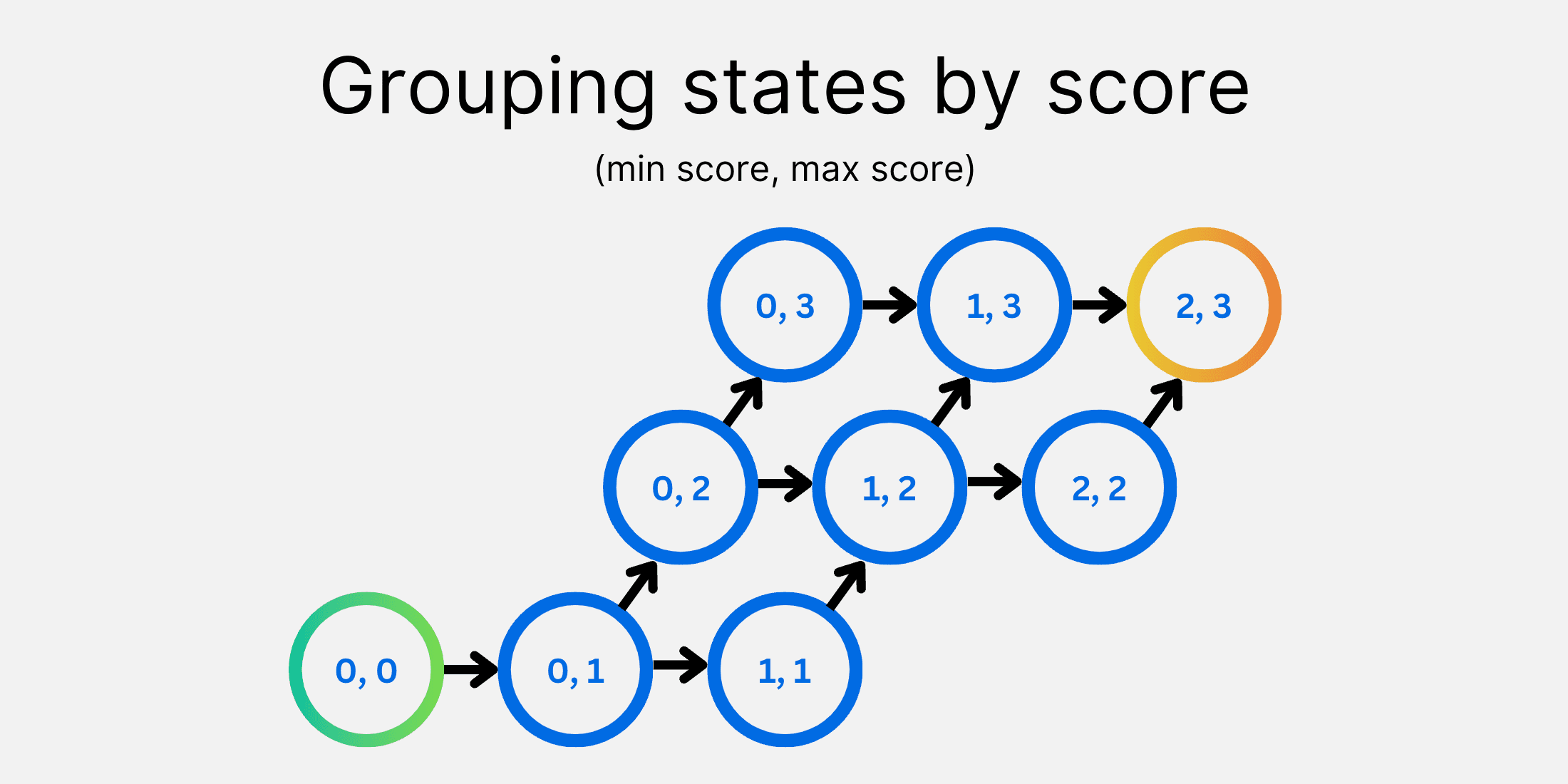
Once you score a piece, you can never unscore it.

Once you score a piece, you can never unscore it. This seemingly inconsequential detail gives us one huge benefit: it breaks all the loops in the state graph. And so, states after a score cannot depend on states before it.

This is a big deal! It allows us to split up the Royal Game of Ur from one big game, down into many smaller "mini-games". Once you score a piece, you progress from one mini-game to the next. We get an advantage in training using this, as each of these mini-games is only dependent upon its own states and states of the next mini-games you could reach.

So instead of training the whole game at once, with all its waste, we are able to train each smaller game one-by-one. And since each of these mini-games is much smaller than the whole game, they can each be trained more efficiently, and with much less waste! This reduces the time it takes to solve the Finkel game from 11 hours to less than 5 hours on my M1 Macbook Pro.

Grouping states of the Royal Game of Ur played with 3 pieces by the number of scored pieces. — The groups we organise states into, the “mini-games”, and their dependencies. The groups shown here represent a ruleset restricted to 3 starting pieces.

We store all the win percentages in a densely-packed map

Another vital consideration for solving the Royal Game of Ur is to make sure we use our memory effectively.

We need a map, or lookup-table, from every position in the game to the likelihood that you would win starting from that position. For the most common Finkel ruleset, this means creating a map of 275,827,872 unique positions. The Masters ruleset is even larger, with over a billion positions to store.

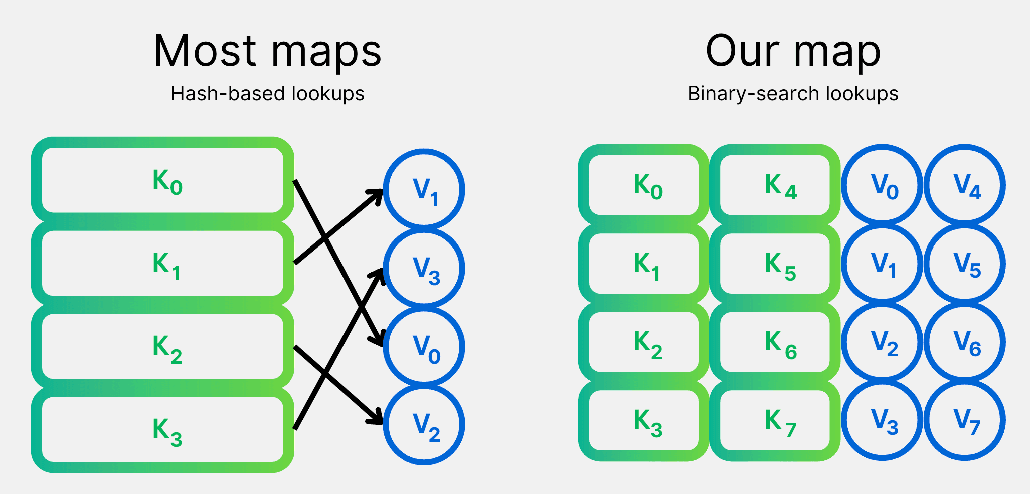
So how do we build these big maps? We decided our best bet was to overcomplicate the process! We were worried about memory, so we built our own map implementation that is optimized for it.

Our maps are made of densely-packed binary keys and values. Instead of the normal approach of hashing keys to find entries, we sort the keys and use binary-search. This allows our maps to be as small as possible, while still being really fast.

Using our overcomplicated map, we are able to keep memory usage down to just 12 bytes per map entry. This means we can store the entire solution for the Finkel ruleset in just 1.6GB. And our compressed versions are as small as 827MB, if accuracy to within 0.01% is good enough for you.

A visualisation of the different memory structures of hash maps and our custom map implementation.

We fit game states into 32-bit keys

The lookup keys in our map represent each position that you can reach in the game. These positions, or states, are snapshots of the game at a fixed point, including whose turn it is, each player's pieces and score, and where all the pieces are on the board. For each of these states, we then store the chance that light wins the game if both players played perfectly from that point onwards.

To use as little memory as possible, we encode the states into small binary numbers. Under the Finkel rule set, we encode states into 32-bits. There is some trickiness to packing all that information in...

The most straightforward way to pack a state into binary, under the Finkel rule set, would leave you with 54-bits:

1-bit: Whose turn is it?
1-bit: Has the game been won?
2 x 3-bits: Light player's pieces and score.
2 x 3-bits: Dark player's pieces and score.
20 x 2-bits: Contents of each tile on the board (tiles can be empty, contain a light piece, or contain a dark piece).

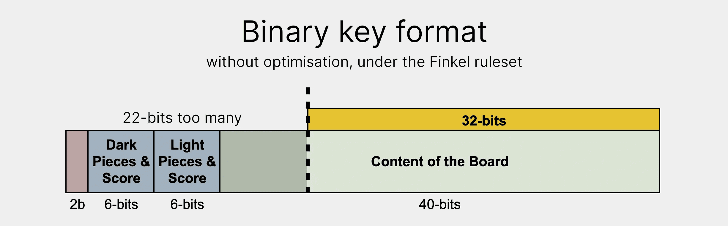
An unoptimised binary format showing 22-bits used past the goal of 32-bits. — A simple, but inefficient, binary format that you could use to encode game states into keys.

54-bit keys aren't so bad. We could use standard long 64-bit numbers to store these keys, and it would still be quite fast and memory efficient. But wouldn't it be nice if we could fit it all in 32-bits instead!

Luckily, there's some simple tricks we have up our sleeves to reduce the number of bits we need.

The first thing we can tackle is that some information in the keys is redundant. The number of pieces players have left to play, and whether the game has been won, can both be calculated from other information we store in the keys. Therefore, we can remove those values and save 7 bits!

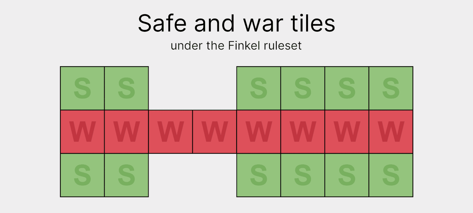
Another 12 bits can also be axed by changing how we store tiles that can only be reached by one player. We call these tiles the "safe-zone" tiles. Since they can only be accessed by one player, we only need 1-bit to store each: 0 for empty, and 1 for containing a piece. This halves the space we need to store these tiles, bringing us down to an overall key-size of 35 bits. That's pretty close to our goal of 32!

The safe-zone and war-zone tiles under the Finkel ruleset of the Royal Game of Ur. — The safe-zone (S) and war-zone (W) tiles under the Finkel ruleset. The safe-zone tiles are green, and the war-zone tiles are red.

The final 3 bits can be removed by compressing the war-zone tiles. Before compression, each war-zone tile uses 2-bits to store its 3 states (empty, light, or dark). That means there's an extra 4th state that 2-bits can represent that we don't use. In other words, an opportunity for compression!

To compress the war-zone, we list out all legal 16-bit variations that the war-zone could take, and assign them to new, smaller numbers using a little lookup table. This allows us to compress the 16 bits down to 13, bringing us to our 32-bit goal!

Ur is symmetrical - symmetrical is Ur

As a cherry on-top, we can also remove the turn bit, as the Royal Game of Ur is symmetrical. This is actually a pretty big deal! It means that if you swap the light and dark players, their chance of winning stays the same. This is really helpful, as it means we only have to store and calculate half the game states. That's a really significant saving!

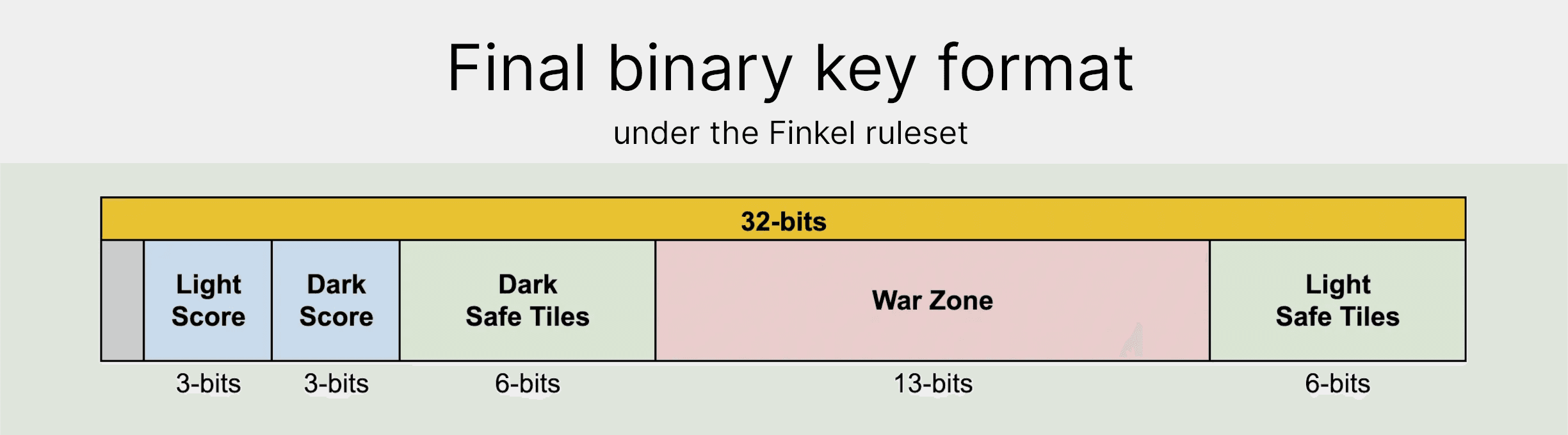
The binary format we use for encoding Finkel game states into keys.

We now have a 31-bit encoding that we can use for the keys in our map! Theoretically, the minimum number of bits we'd need to represent all 137,913,936 states would be 28. So we're a bit off, but I'm pretty happy with getting within 3 bits of perfect!

Other rulesets need more than 32-bits

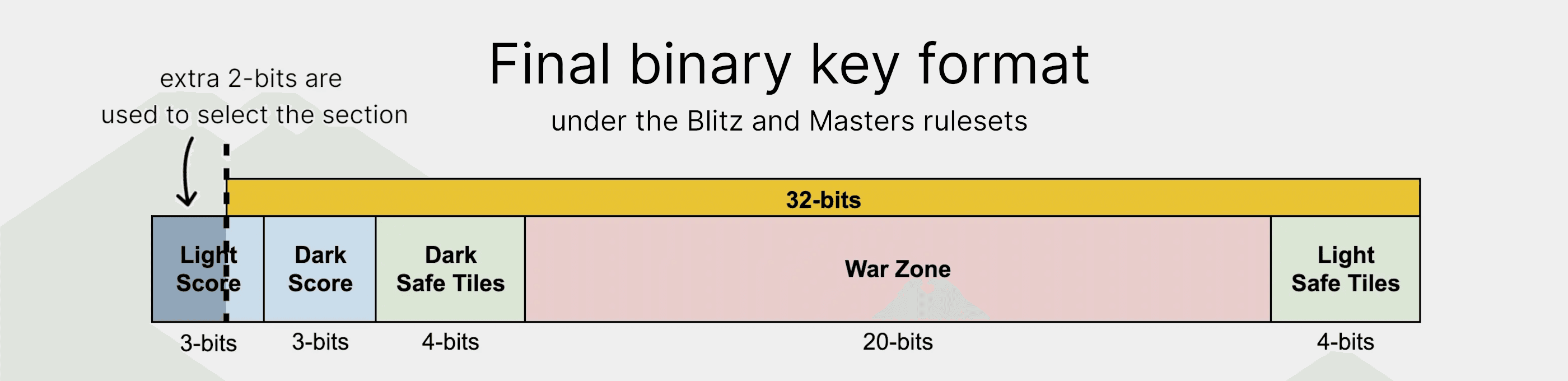
Unfortunately, when we try to move on to different rulesets, we hit a snag. For the Masters and Blitz rulesets the same techniques can only get us down to 34 bits, due to the longer path around the board. That means we have 2 more bits than we wanted...

But our trick bag isn't empty yet! Instead of doubling our key size to 64-bits, we can instead split the map into 4 sections. The 2 extra bits can then be used to select the section to look in, before we search for the actual entry using the remaining 32-bits. This allows us to fit the half a billion entries for the Masters ruleset into 3 GB instead of 5!

The binary format we use for encoding Blitz and Masters game states into keys.

And that's a map, folks! There's nothing too special in our implementation, but it works well for our purposes of reducing memory usage and allowing fast reads and writes.

We open-sourced the solved game

You now have all you need to solve the Royal Game of Ur yourself! Although, if you'd rather experiment with the solved game straight away, we have open-sourced a few different implementations for training and using our models.

The final trained models are available on HuggingFace.
Our Java library, RoyalUr-Java, can read and train these models.
Our Python library, RoyalUr-Python, can read the 16-bit Finkel model.
Jeroen's Julia implementation can really quickly train models that use a different file format.
Raph released the Lut Explorer, which you can use to explore all the different positions in the solved game.

If you do experiment with the solved game, we'd love to hear what you manage to do! If you're interested, I invite you to join our Discord. We have a channel dedicated to discussing research topics, just like everything I've talked about above.

Now, let's zoom-out from the technical details and discuss how solving the Royal Game of Ur fits into the larger landscape of AI.

Can we solve more games?

It's difficult to find a game that aligns as perfectly with value iteration as the Royal Game of Ur. With its element of chance, non-finite gameplay, and limited number of positions, value iteration is the ideal choice for solving the game. Value iteration is rarely as ideal when applied to other games.

Some games we'd love to solve, such as Backgammon, have too many positions for value iteration. Ur has ~276 million positions, while Backgammon contains ~100 quintillion... This means that solving Backgammon using value iteration would require so much storage it verges on the unimaginable. You would need nearly 3% of the world's total data storage, or a trillion gigabytes.

Other popular games, such as Connect-Four or Yahtzee, would be inefficient to solve using value iteration. Connect-Four contains no dice, so it is more efficient to solve using search. Yahtzee has its dice, but it is simplified by its inescapable forwards motion. Once you have made an action in Yahtzee, you can never get back to a state before you took that action. This leads to Yahtzee being more efficient to solve by evaluating the game back to front instead.

We estimate that any game with a state-space complexity on the order of 1E+11 or lower could feasibly be solved using value iteration. This cuts out using value iteration to solve most complex games, including Backgammon.

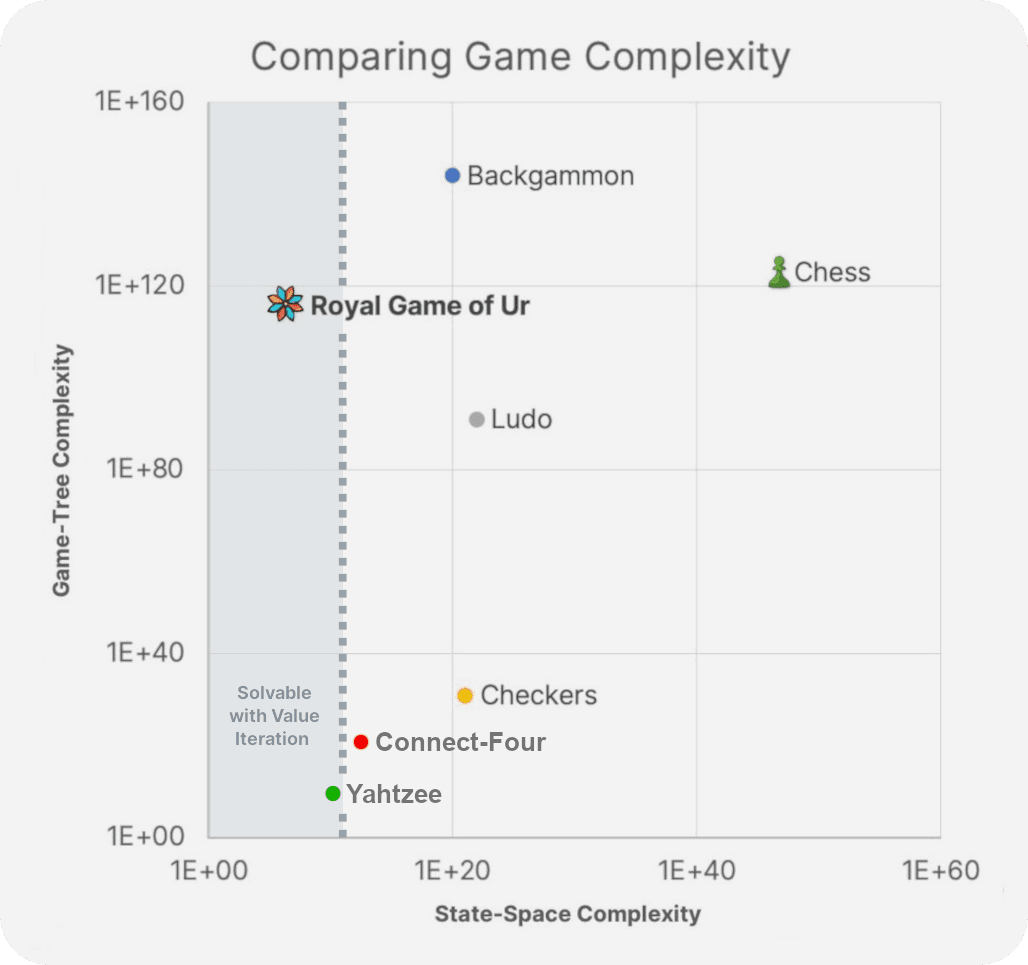
The state-space and game-tree complexity metrics of popular games, including the Royal Game of Ur.

This is why, despite solving Ur being a remarkable achievement for the game, it is not a breakthrough for solving more complex games. There may be some games of chance with perfect information that could be elevated to the title of strongly solved using value iteration. But value iteration alone will not allow us to solve complex games like Backgammon.

Yet, we should not discount value iteration entirely! In the tense final moves of a board game, value iteration can still provide a lot of value. Advanced AI systems for games often rely on databases to play flawlessly in endgames, and value iteration is one method that can be used to build those databases. Bearoff databases, for instance, are commonly used for perfect endgame strategies in Backgammon. Similar techniques could also allow flawless play at the end of other games like Ludo or Parcheesi!

What do we use the solved game for?

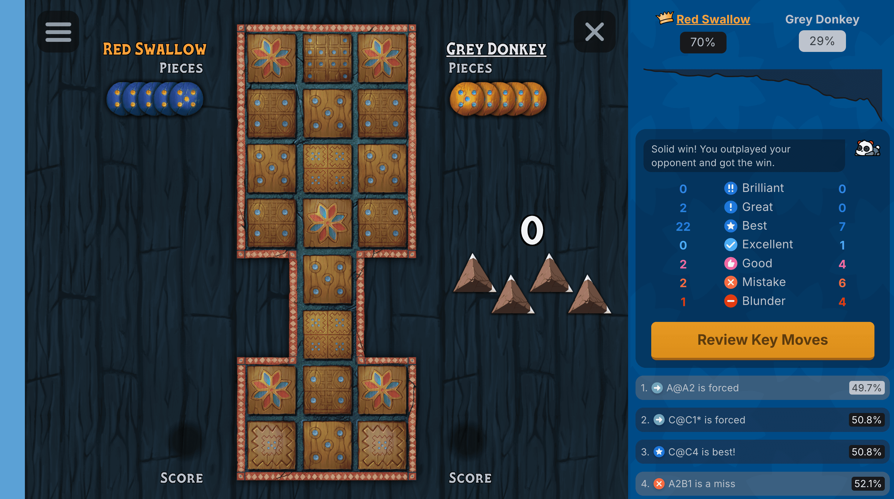
Solving the game allows us to calculate player's accuracy in games, to provide in-depth game reviews, and to let players challenge the perfect player by selecting the Panda as their opponent. This has all had a big impact on how our players play the Royal Game of Ur on our site.

If you're interested to read more about what this means for the Royal Game of Ur, read our blog post about that here.

Thanks for reading!

This was a lot of fun to write, and hopefully you enjoyed reading it as well!

And if you think this is cool, well, I haven't done much else like it. But I have done some other stuff you might find interesting. And if there's any more information you'd like about this project, please reach out! My contact information is on my personal website as well.

Thanks :)
~ Paddy L.